Notes on plotting matrices

Introdution

Accidentally I came across the article written by Yixuan Qiu the link; it’s quite interesting! Inspired by his work, I write down a couple of notes on plotting matrices.

Here I try to answer two questions:

1. How to plot a numeric matrix?
2. How to firstly order rows/columns of a numeric matrix and then plot the ordered matrix?

Plotting a numeric matrix

By a numeric matrix, I mean all its entries are numeric values. Notice that a 0-1 matrix is a numeric matrix.

One way to plot a numeric matrix is to plot each element of the matrix. My ideas are:

• We regard $i$-$j$ entry as a point at $x=j$ and $y=m+1-i$ on a plain, where $m$ is the total number of rows.
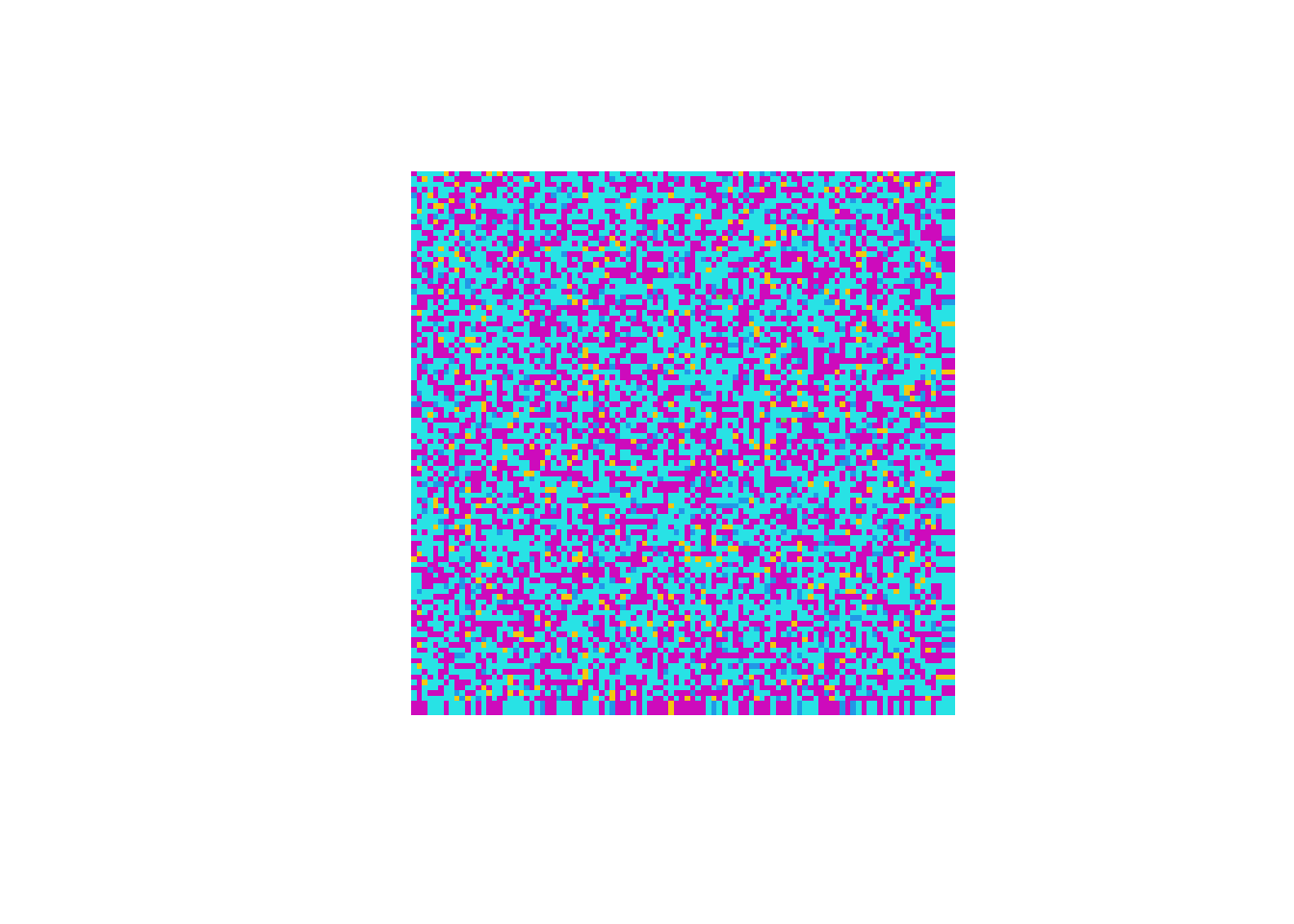
• The value of $i$-$j$ entry is mapped to a color, which is to be shown at point with coordinates $x=j$ and $y=m+1-i$. Here is an example, which is a tweak of an example in Chapter 4 of my book EXPLORING/SOLVING 23 PROBLEMS WITH R.

my_plot_matrix <- function(A, NO_of_col = 7, 
                           the_symbol = 15)
{ # coordinates of an m-by-n matrix
  x_y_coords <- function(m, n)
  {x <- rep(1:n, each = m)
   y <- rep(m:1, times = n) 
   return(data.frame(X = x, Y = y))
  }
  d_x <- dim(A)[1] 
  d_y <- dim(A)[2] 
  the_coords <- x_y_coords(d_x, d_y)
  
  # mapping
  m1 <- min(A)
  ## shifting to make all elements positive
  A <- A + abs(m1) * 2 
  m2 <- max(A)
  ## map to colors
  col_matrix <- ceiling(A / m2 * NO_of_col) 
  
  # plotting
  par(pty = "s") # make the plot region square
  ## create a frame first
  plot(0, 0, 
       xlim = c(0, d_y + 1), 
       ylim=c(0, d_x + 1),
       xlab = "", ylab = "", pch = "", col = 0,
       axes = FALSE, frame.plot = FALSE)
  ## plot all the points
  points(the_coords$X, the_coords$Y, 
         col = col_matrix, 
         pch = the_symbol)
}

set.seed(29052016)
A <- matrix(rnorm(100 * 100), 100, 100)
my_plot_matrix(A)

Ordering rows/columns of a matrix

As for question 2 that I asked in Introduction, here we make the restriction that the matrices are 0-1 ones. We are interested in information in a matrix. If we order rows/columns of the matrix without distortion of the information in the matrix, then we can do so for the purpose of a better way to show the matrix. An example: Suppose matrix $\boldsymbol A$ has $m$ rows and $n$ columns; the rows are for $m$ persons; the columns are for $n$ diseases; $i$-$j$ entry is either 0 or 1, with the meaning that person $i$ has or hasn’t disease $j$. In this example, we have the freedom of ordering the rows (persons) and columns (diseases) without loss of information in the matrix, and doing so we may see “clustering” patterns (in some sense).

To me, ordering a matrix is an interesting problem, and if I have time I probably will read this article Seriation and Matrix Reordering Methods: An Historical Overview—the link is provided in Yixuan Qiu’s article. So for now, following Qiu, I will use R package seriation for ordering matrices.

Another interesting point in Qiu’s article

The first interesting point in Qiu’s article is ordering rows/columns of a 0-1 matrix; this is mentioned in the last section. The other interesting point is that he talks about transforming coordinates of entries with value being equal to 1. For a 0-1 matrix ${\boldsymbol A}=(a_{ij})$, his transformation procedure is as follows.

1. Find where $a_{ij}=1$, i.e. finding the $(i, j)$ indexes.
2. Scale those founded $(i, j)$ indexes: $$ \xi = i/\hbox{max}(i), $$ and $$ \eta = (j-1)/\hbox{max}{(j-1)}\times 2\times \pi. $$
3. Have the transformed coordinates $$ x = \xi \cos(\eta), $$ and $$ y = \xi \sin(\eta). $$

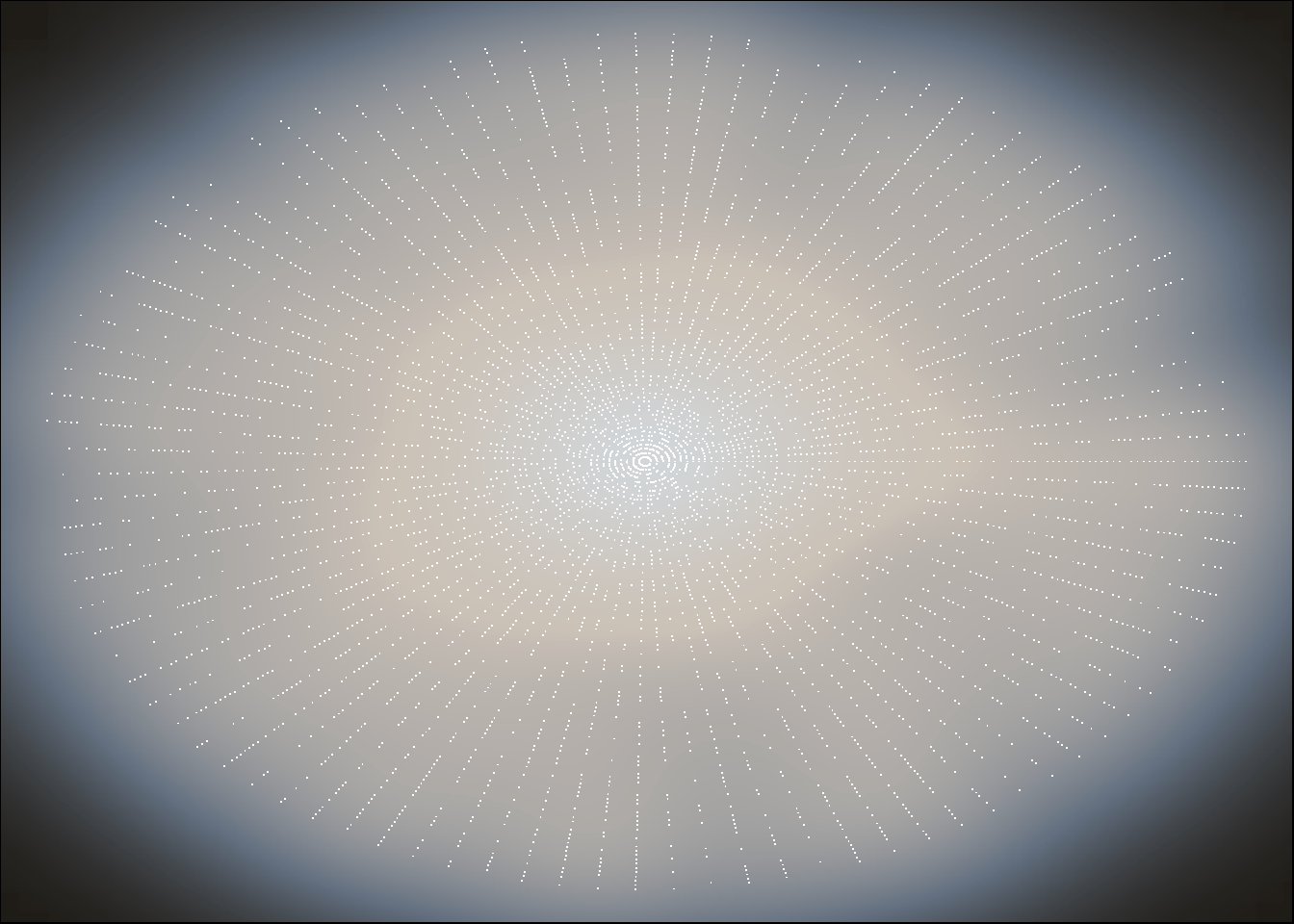
Now let’s have a couple of examples—some amazing pictures will be shown!

Example 1:

# helper functions
coordinate_transform <- function(i, j)
{xi <- i / max(i)
 eta <- (j - 1) / max(j - 1) * 2 *pi
 x <- xi * cos(eta)
 y <- xi * sin(eta)
 return(data.frame(X = x, Y = y))
}

plot_func <- function(a_matrix)
{ord <-  seriation::seriate(x = (a_matrix > 0)) 
 ordered_matrix <- seriation::permute(a_matrix, ord)
 coord <- which(ordered_matrix > 0, arr.ind = TRUE) 
 coord_df <- coordinate_transform(i = coord[, "row"], 
                                  j = coord[, "col"])
 # the following lines of code are from Yixuan Qiu
 # par(bg = "black", mar = c(0, 0, 0, 0))
 # plot(coord_df$X, coord_df$Y, col = "white", pch = ".")
 par(bg = "black", mar = c(0, 0, 0, 0))
 mypalette <-  
   colorRampPalette(c("#1F1C17", "#637080",
                      "#CBC2B7", "#D2D6D9"),
                    space = "Lab")
 smoothScatter(coord_df$X, 
               coord_df$Y, 
               colramp = mypalette, 
               nbin = 600, bandwidth = 0.1,
               col = "white", nrpoints = Inf)
}

# generate data
set.seed(20220306)
data_1 <- 
  data.frame(x = sample(letters[1:5], 100, replace = TRUE),
             y = sample(LETTERS[1:5], 100, replace = TRUE),
             stringsAsFactors = FALSE)
frq_matrix <- as.data.frame.matrix(table(data_1$x, data_1$y))
plot_func(frq_matrix)

Example 2:

data_2 <- matrix(rnorm(100*100), 100, 100)
plot_func(data_2)