Notes on One-Stage Clustering Sampling

Introduction

Recently, I reread Chapter 5, “Cluster Sampling with Equal Probabilities”, from Professor Lohr’s book [1]. Here, I want to write down some notes that I found interesting—at least to me.

ICC, adjusted R-squared, and design effect

I am talking about one-stage clustering sampling, and I make the following assumptions:

• There are $N$ clusters in the population.
• Each cluster has $M$ units in it.
• The key variable is $y$, and $y_{ij}$ is the value of unit $j$ in cluster $i$.

We first define

$$ \bar{y} := \frac{\sum_{i=1}^N\sum_{j=1}^M y_{ij}}{NM}, $$

and

$$ y_{i.} := \frac{\sum_{j=1}^M y_{ij}}{M}. $$

Then we can define the three sums of squares:

$$ \hbox{SSTo} := \sum_{i=1}^N\sum_{j=1}^M (y_{ij} - \bar{y})^2; $$

$$ \hbox{SSB} := \sum_{i=1}^N\sum_{j=1}^M (y_{i.} - \bar{y})^2; $$

$$ \hbox{SSW} := \sum_{i=1}^N \sum_{j=1}^M (y_{ij} - y_{i.})^2. $$

Next, we can have the corresponding means:

$$ S^2 := \frac{\hbox{SSTo}}{NM - 1}; $$

$$ \hbox{MSB} := \frac{SSB}{N-1}; $$

$$ \hbox{MSW} := \frac{SSW}{N(M-1)}. $$

In [1], the Intraclass Correlation Coefficient is defined as

$$ \hbox{ICC} := 1 - \frac{M}{M-1}\frac{\hbox{SSW}}{\hbox{SSTo}}; $$

and the adjusted R-squared is defined as

$$ R^2_a := 1 - \frac{\hbox{MSW}}{S^2}. $$

Phew, a lot of math typing! But so far it’s just preparation.

It states in [1] that “$R^2_a$ is close to $\hbox{ICC}$”, and now I show how they are closely related to each other. Notice that

$$ \begin{aligned} \hbox{ICC} & = 1 - \frac{M}{M-1}\frac{\hbox{SSW}}{\hbox{SSTo}}\\ & = 1 - \frac{M}{M-1}\frac{N(M-1)\hbox{MSW}}{(NM-1)S^2}\\ & = 1 - \frac{NM}{NM-1}\frac{\hbox{MSW}}{S^2}. \end{aligned} $$

It follows from the above that

$$ R^2_a - \hbox{ICC} = \frac{1}{NM - 1}\frac{\hbox{MSW}}{S^2} > 0. $$

Important: $R^2_a$ is always greater than $\hbox{ICC}$. Both $\hbox{ICC}$ and $R^2_a$ can be negative.

The reason that [1] introduces $\hbox{ICC}$ and $R^2_a$ is to use them to express the design effect—denoted by $d_{\hbox{eff}}$—of one-stage cluster sampling. In [1], it shows that

$$ d_{\hbox{eff}} = \frac{MSB}{S^2}, $$

and that

$$ d_{\hbox{eff}} = 1 + \frac{N(M-1)}{N-1}R^2_a \approx 1 + (M-1)R^2_a, $$

and that

$$ d_{\hbox{eff}} = \frac{NM-1}{M(N-1)}[1 + (M-1)\hbox{ICC}] \approx 1 + (M-1) \hbox{ICC}. $$

Important: $1 + (M-1)R^2_a$ and $1 + (M-1) \hbox{ICC}$ are very good approximations to $d_{\hbox{eff}}$.

More on $\hbox{ICC}$

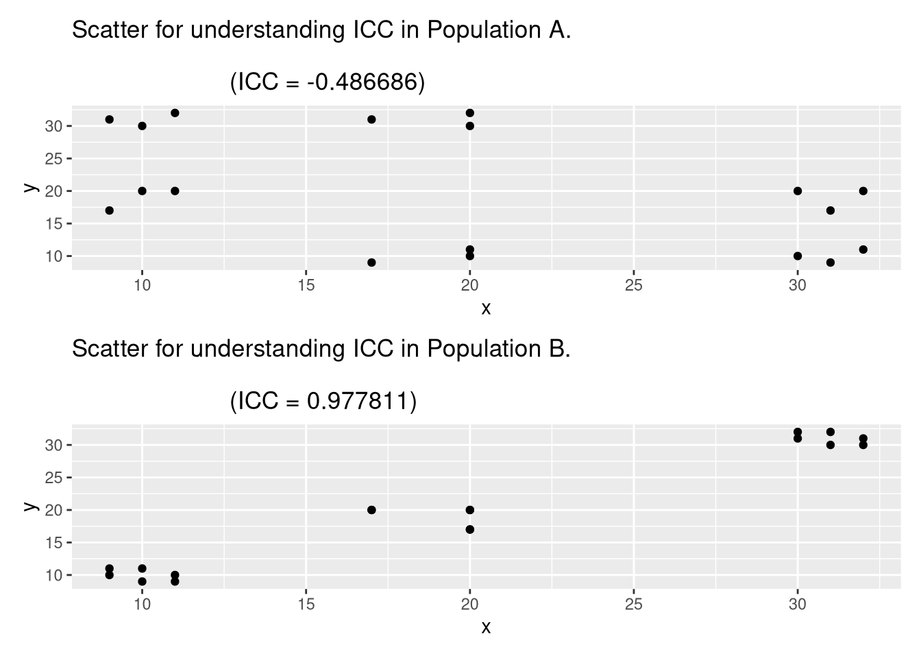
A useful statement from [1] is: “The $\hbox{ICC}$ is defined to be the Pearson correlation coefficient for the $NM(M − 1)$ pairs $(y_{ij}, y_{ik})$ for $i$ between 1 and $N$ and $j \neq k$.” Using this information, I wrote following R code (with help from MS 365 Pilot) to help visually understand $\hbox{ICC}$.

library(tidyverse)
library(patchwork)

cross_within_group <- function(df) {
  df %>%
    inner_join(df, by = "group", suffix = c("_x", "_y"),
               relationship = "many-to-many") %>%
    filter(ID_x != ID_y) %>%
    transmute(x = v_x, y = v_y)
}

# Population A shown in Table 5.4 of [1]
P_A <-  
  data.frame(ID = 1:9,
             group = rep(1:3, each = 3),
             v = c(10, 20, 30, 11, 20, 32, 9, 17, 31))
re_A <- cross_within_group(P_A)
(ICC_A <- cor(re_A$x, re_A$y))

## [1] -0.4866864

plot_a <-
  re_A |>
  ggplot(aes(x = x, y = y)) +
  geom_point() +
  labs(title = sprintf("Scatter for understanding ICC in Population A.\n
                       (ICC = %f)", ICC_A))

# Population B shown in Table 5.4 of [1]
P_B <-  
  data.frame(ID = 1:9,
             group = rep(1:3, each = 3),
             v = c(9, 10, 11, 17, 20, 20, 31, 32, 30))
re_B <- cross_within_group(P_B)
(ICC_B <- cor(re_B$x, re_B$y))

## [1] 0.9778107

plot_b <-
  re_B |>
  ggplot(aes(x = x, y = y)) +
  geom_point() +
  labs(title = sprintf("Scatter for understanding ICC in Population B.\n
                       (ICC = %f)", ICC_B))

plot_a / plot_b

Lumley’s insights

Last year, I came across Professor Thomas Lumley’s blog post, and now I would like to share the following quotes:

Strata are a partition of the population where we hope different strata are different. We sample from all the strata in the population, so the generalisation from the sample to the population is within strata and is more accurate because of stratified sampling.

Clusters are a partition of the population where we fear different clusters are different. We are forced to sample from just a few clusters in the population, because it’s cheaper that way. The generalisation from the sample to the population is between clusters and is less accurate because of cluster sampling.

References

[1] Lohr, S. L. (2022). Sampling: Design and Analysis, 3rd Edition. pp. 167-179.