A Note on Reducing Bais With Delete-1 Jackknife
Introduction
We consider the model: $X_1, X_2, \ldots, X_n$ are independent and identically distributed random variables. Let $\theta$ be the distribution parameter that we want to estimate based on a sample
$$ {\boldsymbol X}=\{X_1=x_1, \ldots, X_n=x_n\}. $$
Here $\theta$ is a generic one, e.g. it can be the mean or the variance or another distribution parameter. Suppose we have an estimator $$ \hat{\theta}= g({\boldsymbol X}). $$
Delete-1 Jackknife resampling procedure results in $n$ Jackknife samples, denoted by $JK_i$ for $i=1, \ldots, n$, where $JK_i$ is the same as the original sample except that it does not include $x_i$. Using $JK_i$, we have a Jackknife estimator $$ \hat{\theta}_{(i)}=g(JK_i). $$
The bias of $\hat{\theta}$ is $$ \hbox{bias}\left(\hat{\theta}\right)=E\left(\hat{\theta}\right)-\theta. $$ The estimator of $\hbox{bias}\left(\hat{\theta}\right)$, which is called Jackknife bias, is
$$ (n-1)\left(\hat{\theta}_{(\cdot)}-\hat{\theta}\right), $$ where
$$ \hat{\theta}_{(\cdot)}=\frac{1}{n}\sum_{i=1}^n\hat{\theta}_{(i)}. $$
Reference paper [1] explains why using multiplier $n-1$ in the estimator of $\hbox{bias}\left(\hat{\theta}\right)$.
Define
$$ \begin{array}{lcl} \hat{\theta}_{\hbox{jack}}&=&\hat{\theta}-(n-1)\left(\hat{\theta}_{(\cdot)}-\hat{\theta}\right)\\ &=& n\hat{\theta}-(n-1)\hat{\theta}_{(\cdot)}. \end{array} $$
According to [1], it’s not true that always
$$ \hbox{bias}(\hat{\theta}_{\hbox{jack}}) = 0 $$
but$$ |\hbox{bias}(\hat{\theta}_{\hbox{jack}})| < |\hbox{bias}(\hat{\theta})| \ \hbox{asymptotically}. $$
Examples
Example 1: $\theta$ is the mean
In this case
$$ \begin{array}{lcl} \hat{\theta}&=&\sum_{i=1}^n x_i/n,\\ \hat{\theta}_{(\cdot)}&=&\hat{\theta},\\ \hat{\theta}_{\hbox{jack}}&=&\hat{\theta}. \end{array} $$
Example 2: $\theta$ is the variance
Let $$ \bar{x}=\frac{1}{n}\sum_{i=1}^n x_i. $$ In this case, if we let $$ \hat{\theta}=\frac{1}{n}\sum_{i=1}^n(x_i-\bar{x})^2, $$ then the Jackknife bias is
$$ (n-1)\left(\hat{\theta}_{(\cdot)}-\hat{\theta}\right)=-\frac{1}{n}\frac{1}{n-1}\sum_{i=1}^n(x_i-\bar{x})^2 $$
and $$ \hat{\theta}_{\hbox{jack}}=\frac{1}{n-1}\sum_{i=1}^n(x_i-\bar{x})^2, $$ which is a pleasant surprise because it is the same as the commonly used sample variance.Example 3: $X_1\sim \hbox{Uniform}(0, \theta)$
Define $$ x_{(n)}=\hbox{max}\left({x_1, \ldots, x_n}\right), $$ and
$$ x_{(n-1)}=\hbox{max}\left(\{x_1, \ldots, x_n\}\backslash \{x_{(n)}\}\right). $$
In this case, $$ \hat{\theta}=x_{(n)}, $$ and$$ \hat{\theta}_{(\cdot)}=\frac{n-1}{n}x_{(n)}+\frac{1}{n}x_{(n-1)}, $$
and the Jackknife bias is $$ -\frac{n-1}{n}\left(x_{(n)}-x_{(n-1)}\right), $$ and $$ \hat{\theta}_{\hbox{jack}}=x_{(n)}+\frac{n-1}{n}\left(x_{(n)}-x_{(n-1)}\right). $$ Using the results in Appendix, we can show that under the assumption$X_1\sim \hbox{Uniform}(0, \theta)$,
$$ \begin{array}{lcl} E\left(x_{(n)}\right)&=&\frac{n}{n+1}\theta<\theta,\\ E\left(x_{(n-1)}\right)&=&\frac{n-1}{n+1}\theta. \end{array} $$
Thus, $$ E\left(\hat{\theta}_{\hbox{jack}}\right)=\frac{n^2+n-1}{n^2+n}\theta<\theta. $$ It is obvious that$$ E\left(\hat{\theta}\right) < E\left(\hat{\theta}_{\hbox{jack}}\right) < \theta. $$
We next construct the following estimators
$$ \hat{\theta}_1=\hat{\theta}, $$
and unbiased estimators:$$ \hat{\theta}_2 = \frac{n+1}{n}\hat{\theta}, $$
$$ \hat{\theta}_3 = \frac{n^2+n}{n^2+n-1}\hat{\theta}_{\hbox{jack}}, $$
and$$ \hat{\theta}_4 = 2x_{(n)}-x_{(n-1)}. $$
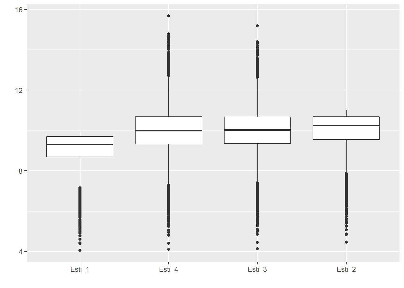
To understand the relative performances of the above four estimators, we do simulations with the following R code:library(dplyr)
library(tidyr)
library(ggplot2)
# a function factory
estimator <- function(esti)
{function(x) {
n <- length(x)
ordered_x <- sort(x)
x_ <- ordered_x[n]
x__ <- ordered_x[n-1]
switch (esti,
"1" = x_,
"2" = (n + 1) / n * x_,
"3" = (2 * n^2 + n - 1) / (n^2 + n - 1) * x_ -
(n^2 - 1) / (n^2 + n - 1) * x__,
"4" = 2 * x_ - x__,
stop("Invalid `esti` value")
) }
}
# put N samples of size n into an N-by-n matrix
create_samples <- function(N = 10000, n = 10, theta = 10) {
matrix(runif(n * N, min = 0, max = theta), ncol = n, nrow = N, byrow = TRUE)
}
# a simulator
simulator <- function(N = 10000, n = 10)
{the_samaples <- create_samples(N = N, n = n)
the_estimates <- matrix(0, nrow = N, ncol = 4)
for(i in 1:4) {
the_fun <- estimator(as.character(i))
the_estimates[, i] <- apply(the_samaples, 1, the_fun)
}
chk_the_means <- apply(the_estimates, 2, mean)
chk_the_vars <- apply(the_estimates, 2, var)
chk_mse <- apply(the_estimates, 2, function(x) mean(sum((x - 10)^2)))
df <-
as.data.frame(the_estimates) %>%
pivot_longer(cols = V1:V4, names_to = "estimator", values_to = "estimate") %>%
mutate(estimator = recode(estimator,
V1 = "Esti_1",
V2 = "Esti_2",
V3 = "Esti_3",
V4 = "Esti_4"))
p <-
ggplot(df) +
geom_boxplot(aes(x = reorder(estimator, estimate, FUN = median),
y = estimate)) +
labs(x = "", y = "")
list(chk_the_means, chk_the_vars, chk_mse, p)
}
# simulations
set.seed(20220807)
## n = 10
simu_n_10 <- simulator(n = 10)
(simu_n_10[1:3])
## [[1]]
## [1] 9.074361 9.981797 9.985849 9.986258
##
## [[2]]
## [1] 0.7009157 0.8481080 1.4215333 1.5420883
##
## [[3]]
## [1] 15576.526  8483.545 14215.914 15421.230
(simu_n_10[4])
## [[1]]

## n = 100
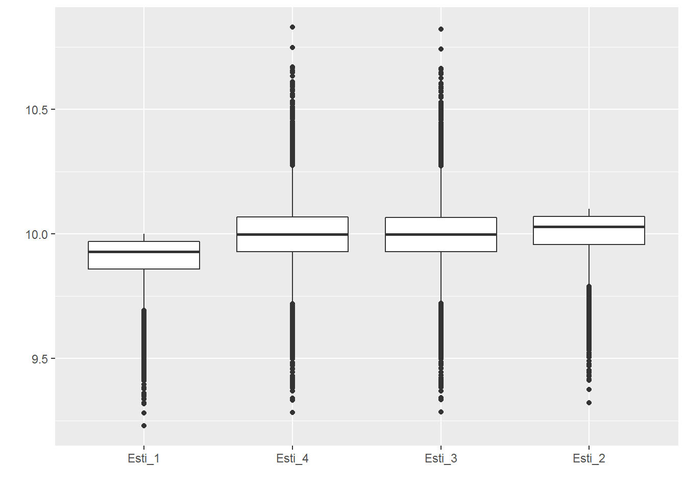
simu_n_100 <- simulator(n = 100)
(simu_n_100[1:3])
## [[1]]
## [1] 9.899993 9.998993 9.998263 9.998256
##
## [[2]]
## [1] 0.009463968 0.009654193 0.018759910 0.018943620
##
## [[3]]
## [1] 194.64411  96.54242 187.61051 189.44768
(simu_n_100[4])
## [[1]]

Based on the above, we can conclude that $\hat{\theta}_2$ is the best among the four estimators.
Appendix
$X_1, X_2, \ldots, X_n$ are independent and identically distributed random variables. The probability density function (PDF) and cumulative distribution function (CDF) are $f(x)$ and $F(x)$, respectively. Let $X_{(n)}$ and $X_{(n-1)}$ be the largest and the second largest, respectively, among $X_1, X_2, \ldots, X_n$. Then the PDFs of $X_{(n)}$ and $X_{(n-1)}$ are $$ f_{(n)}(x)=nF(x)^{n-1}f(x), $$ and $$ f_{(n-1)}(x)=n(n-1)[1-F(x)]F(x)^{n-2}f(x). $$
Proof: The CDF of $X_{(n)}$ is
$$ \begin{array}{ccl} F_{(n)}(x)&=&P(X_{(n)}\le x)\\ &=&P(X_1\le x, \cdots, X_n \le x)\\ &=& F(x)^n. \end{array} $$
Taking derivative, we have the desired result.The CDF of $X_{(n-1)}$ is
$$ \begin{array}{ccl} F_{(n-1)}(x)&=&P(X_{(n-1)}\le x)\\ &=&P(X_{(n-1)}\le x\ \hbox{and}\ X_{(n)}\le x) +\\ & &P(X_{(n-1)}\le x\ \hbox{and}\ X_{(n)}> x)\\ &=&P(X_{(n)}\le x)+nP(X_1\le x, \ldots, X_{n-1}\le x, X_n>x)\\ &=& F(x)^n + nF(x)^{n-1}[1-F(x)]. \end{array} $$
Taking derivative, we complete the proof.References
[1] McIntosh, A. The Jackknife Estimation Method. URL: https://arxiv.org/pdf/1606.00497.pdf