Finding Maximum and Range: Two Exercises

Exercise 1

In my leisure time, I often watch YouTube videos that I am interested in. One day, I came cross a video, which teaches how to solve the following math problem:

Given that $x^2+y^2=1$, find the maximum of

$$ z = (x+1)(y+2). $$

When I saw the problem, I started to give an analytic solution but no success. Then I went back to the video, for some reason, it’s gone and I cannot find it any more!? OK, here I wrote the following R code to solve the problem.

# method 1
obj_fun <- function(x)
{y <- sqrt(1 - x^2)
 (x + 1) * (y + 2)
}

N <- 1e4
x <- seq(0, 1, length.out = N)
y <- obj_fun(x)

plot(x, y, pch = '.', ylab = 'obj_function')

the_index <- which(y == max(y))
x_coordinate <- x[the_index]
y_coordinate <- sqrt(1 - x_coordinate^2)
abline(v = x_coordinate, lty = 2, col = 'blue')
abline(h = y[the_index], lty = 2, col = 'blue')

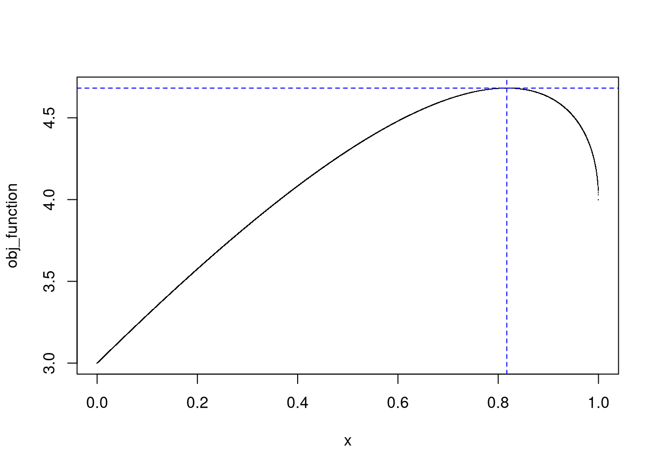
(list(x_coordinate, y_coordinate, y[the_index]))

## [[1]]
## [1] 0.8171817
## 
## [[2]]
## [1] 0.5763801
## 
## [[3]]
## [1] 4.681751

# method 2
library(rootSolve) 
theta_func <- function(theta)
{cos(theta) - 2 * sin(theta) + cos(2*theta)
}

curve(theta_func, 0.0, pi/2)
abline(h = 0, col = 'red')

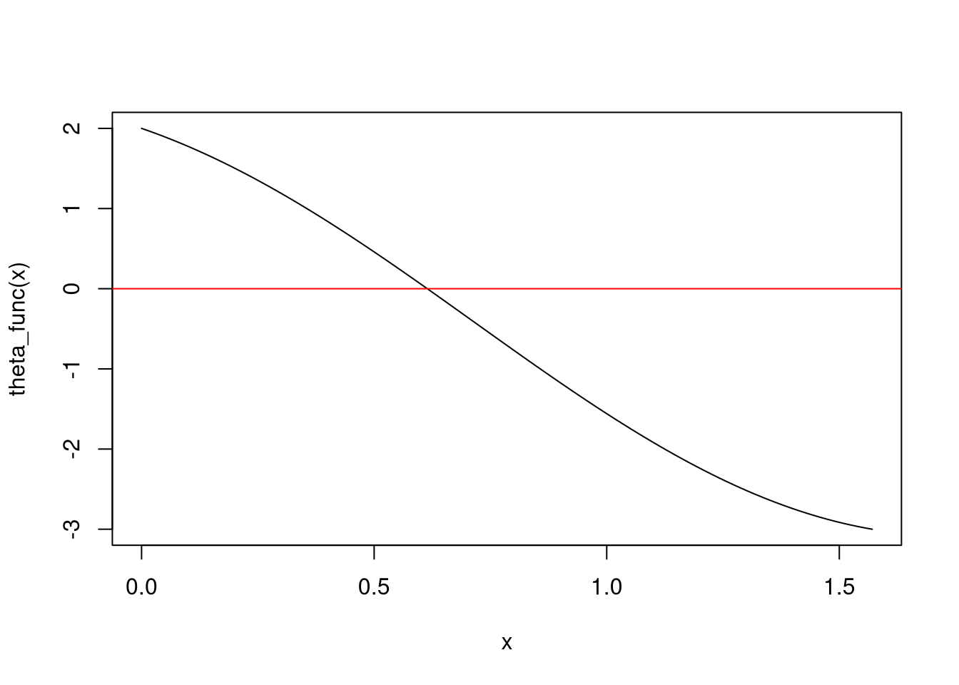
the_root <- uniroot(theta_func, c(0.5, 1.0), tol = 1e-8)$root
x <- cos(the_root)
y <- sin(the_root)
the_max <- (x + 1) * (y + 2)
list(x, y, the_max)

## [[1]]
## [1] 0.8171826
## 
## [[2]]
## [1] 0.5763788
## 
## [[3]]
## [1] 4.681751

Exercise 2

The second math problem also comes from YouTube.

We are given:

• $a,\ b,\ c >0$
• $abc = 8$

What is the range of

$$ S = \frac{1}{\sqrt{1+a}} + \frac{1}{\sqrt{1+b}} + \frac{1}{\sqrt{1+c}}? $$

I did listen to the YouTube video, but I felt the solution is quite complicated. So, today, I asked Microsoft 365 (M365) Copilot to give me an answer. M365 Copilot did a good job, it pointed out that

• $f(x) = \frac{1}{\sqrt{1+x}}$ is a decreasing function;
• the key to solve the problem is to let $a$ (or $b$ or $c$) get close to 0 or $+\infty$

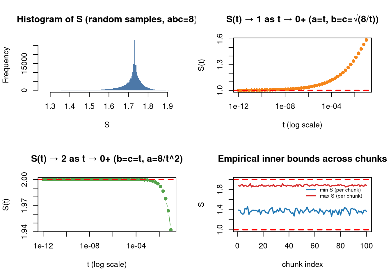
So the answer is: $S \in (1, 2)$.

Next I asked M365 Copilot to write R code to show numerical evidence that the range of $S$ is $(0,\ 1)$. Below is the code that was written by M365 Copilot (with minor changes that I did.) To be honest, the code is not bad!

# ---------------------------------------------
# Empirical evidence that S ∈ (1, 2) for a,b,c>0 with abc = 8
# ---------------------------------------------

# Helper: S(a,b,c)
S_val <- function(a, b, c) {
  1 / sqrt(1 + a) + 1 / sqrt(1 + b) + 1 / sqrt(1 + c)
}

# ---------------------------------------------
# 1) Random sampling under the constraint abc = 8
# ---------------------------------------------
# We sample (u, v) freely in R, set w = -(u+v) to force u+v+w = 0,
# then define: a = 8*exp(u), b = exp(v), c = exp(w).
# This ensures a, b, c > 0 and a*b*c = 8*exp(u+v+w) = 8.

set.seed(123)
n <- 200000

u <- rnorm(n, mean = 0, sd = 1.0)
v <- rnorm(n, mean = 0, sd = 1.0)
w <- -(u + v)

a <- 8 * exp(u)
b <- exp(v)
c <- exp(w)

S <- S_val(a, b, c)

cat("RANDOM SAMPLING SUMMARY (abc=8):\n")

## RANDOM SAMPLING SUMMARY (abc=8):

cat(sprintf("  min(S) ≈ %.6f\n", min(S)))

##   min(S) ≈ 1.263860

cat(sprintf("  1st quartile ≈ %.6f, median ≈ %.6f, 3rd quartile ≈ %.6f\n",
            quantile(S, 0.25), quantile(S, 0.5), quantile(S, 0.75)))

##   1st quartile ≈ 1.704253, median ≈ 1.730939, 3rd quartile ≈ 1.745701

cat(sprintf("  max(S) ≈ %.6f\n\n", max(S)))

##   max(S) ≈ 1.916738

# Check if any sample violates 1 < S < 2 (should be none for large n, within numeric tolerance)
eps <- 1e-12
viol_lo <- sum(S <= 1 + eps)
viol_hi <- sum(S >= 2 - eps)
cat(sprintf("Violations count (S ≤ 1+%.0e): %d\n", eps, viol_lo))

## Violations count (S ≤ 1+1e-12): 0

cat(sprintf("Violations count (S ≥ 2-%.0e): %d\n\n", eps, viol_hi))

## Violations count (S ≥ 2-1e-12): 0

# ---------------------------------------------
# 2) Constructive sequences approaching endpoints
# ---------------------------------------------

# 2A) Approach 1 from above:
# Take a = t → 0+, and choose b = c = sqrt(8/t) so that abc = 8.
# Then S(t) = 1/sqrt(1+t) + 2/sqrt(1 + sqrt(8/t)) → 1 as t → 0+.
t_vals_small <- 10^seq(-12, -1, length.out = 50)
S_to_1 <- sapply(t_vals_small, function(t) {
  a <- t
  b <- c <- sqrt(8 / t)
  S_val(a, b, c)
})

cat("APPROACH TO 1 FROM ABOVE:\n")

## APPROACH TO 1 FROM ABOVE:

cat(sprintf("  min S(t) on grid ≈ %.12f (t_min = %.1e)\n\n",
            min(S_to_1), t_vals_small[which.min(S_to_1)]))

##   min S(t) on grid ≈ 1.001189206904 (t_min = 1.0e-12)

# 2B) Approach 2 from below:
# Take b = c = t → 0+, and a = 8/t^2 so that abc = 8.
# Then S(t) = 1/sqrt(1 + 8/t^2) + 2/sqrt(1 + t) → 2 as t → 0+.
t_vals_zero <- 10^seq(-12, -1, length.out = 50)
S_to_2 <- sapply(t_vals_zero, function(t) {
  b <- c <- t
  a <- 8 / (t^2)
  S_val(a, b, c)
})

cat("APPROACH TO 2 FROM BELOW:\n")

## APPROACH TO 2 FROM BELOW:

cat(sprintf("  max S(t) on grid ≈ %.12f (t_min = %.1e)\n\n",
            max(S_to_2), t_vals_zero[which.max(S_to_2)]))

##   max S(t) on grid ≈ 1.999999999999 (t_min = 1.0e-12)

# ---------------------------------------------
# 3) Optional: Visualizations
# ---------------------------------------------
do_plots <- TRUE
if (do_plots) {
  oldpar <- par(no.readonly = TRUE)
  on.exit(par(oldpar), add = TRUE)
  par(mfrow = c(2, 2))
  
  # Histogram of S from random sampling
  hist(S, breaks = 100, col = "#4C78A8", border = NA,
       main = "Histogram of S (random samples, abc=8)",
       xlab = "S", xlim = c(min(S), max(S)))
  # abline(v = c(1, 2), col = c("red", "red"), lwd = 2, lty = 2)
  # abline(v = sqrt(3), col = "darkgreen", lwd = 2, lty = 3)
  # legend("topright", legend = c("S = 1", "S = 2", "S = √3 (a=b=c=2)"),
  #       col = c("red", "red", "darkgreen"), lty = c(2, 2, 3), bty = "n")
  
  # S(t) approaching 1
  plot(t_vals_small, S_to_1, type = "b", log = "x", pch = 16, col = "#F58518",
       main = "S(t) → 1 as t → 0+ (a=t, b=c=√(8/t))",
       xlab = "t (log scale)", ylab = "S(t)")
  abline(h = 1, col = "red", lwd = 2, lty = 2)
  
  # S(t) approaching 2
  plot(t_vals_zero, S_to_2, type = "b", log = "x", pch = 16, col = "#54A24B",
       main = "S(t) → 2 as t → 0+ (b=c=t, a=8/t^2)",
       xlab = "t (log scale)", ylab = "S(t)")
  abline(h = 2, col = "red", lwd = 2, lty = 2)
  
  # Scatter of (min(S), max(S)) from random sampling subsets
  # (just to illustrate empirical inner bounds tightening with more samples)
  chunk <- 2000
  k <- floor(n / chunk)
  mins <- numeric(k); maxs <- numeric(k)
  for (i in 1:k) {
    idx <- (((i - 1) * chunk) + 1):(i * chunk)
    mins[i] <- min(S[idx]); maxs[i] <- max(S[idx])
  }
  
  
  y_range <- range(c(mins, maxs), na.rm = TRUE, finite = TRUE)
  
  tiny_nbr <- 1e-8
  
  plot(1:k, mins, type = "l",
       col = "#1F77B4", lwd = 2,
       ylim = c(1 - tiny_nbr, 2 + tiny_nbr),
       main = "Empirical inner bounds across chunks",
       xlab = "chunk index", ylab = "S")
  
  lines(1:k, maxs,
        col = "#D62728", lwd = 2)
  
  abline(h = c(1, 2), col = "red", lwd = 2, lty = 2)
  
  # Place legend at 90% of the x-range and 97% of the y-range
  x_pos <- 0.5 * k
  y_pos <- y_range[1] + 1.0 * diff(y_range)
  
  legend(x_pos, y_pos,
         legend = c("min S (per chunk)", "max S (per chunk)"),
         col = c("#1F77B4", "#D62728"),
         lwd = 2, lty = 1, bty = "n", cex = 0.65)
  
}

# ---------------------------------------------
# 4) Sanity checks at special points
# ---------------------------------------------
# Symmetric point a=b=c=2 (abc=8): S = sqrt(3)
S_sym <- S_val(2, 2, 2)
cat(sprintf("Symmetric point (a=b=c=2): S = %.12f (should be √3 ≈ %.12f)\n",
            S_sym, sqrt(3)))

## Symmetric point (a=b=c=2): S = 1.732050807569 (should be √3 ≈ 1.732050807569)

# A configuration near the lower endpoint (S ~ 1)
# Choose very small t
t <- 1e-9
S_near1 <- S_val(t, sqrt(8/t), sqrt(8/t))
cat(sprintf("Near lower endpoint: t=%.1e → S ≈ %.12f (approaches 1 from above)\n",
            t, S_near1))

## Near lower endpoint: t=1.0e-09 → S ≈ 1.006687365166 (approaches 1 from above)

# A configuration near the upper endpoint (S ~ 2)
t <- 1e-9
S_near2 <- S_val(8/(t^2), t, t)
cat(sprintf("Near upper endpoint: t=%.1e → S ≈ %.12f (approaches 2 from below)\n",
            t, S_near2))

## Near upper endpoint: t=1.0e-09 → S ≈ 1.999999999354 (approaches 2 from below)

cat("\nConclusion: Random sampling shows 1 < S < 2, and constructive families show\n")

## 
## Conclusion: Random sampling shows 1 < S < 2, and constructive families show

cat("S can get arbitrarily close to 1 and 2 without reaching them. Thus S ∈ (1, 2).\n")

## S can get arbitrarily close to 1 and 2 without reaching them. Thus S ∈ (1, 2).